


Research theoretical foundation
The theoretical foundation of this work lies primarily at the intersection of strategic management and AI technology. First, strategic management theory provides the decision-making framework and guiding principles for this work18. Strategic management involves the processes by which enterprises analyze, formulate, implement, and evaluate strategies to achieve their long-term goals and sustainable development in a competitive environment. Classic strategic management theories include Porter’s Competitive Advantage Theory, the Resource-Based View (RBV), and Dynamic Capabilities Theory. These theories offer a theoretical basis for how enterprises can maintain competitiveness in a complex and ever-changing market environment19,20.
Porter’s Competitive Advantage Theory emphasizes that enterprises should achieve competitive advantage through three basic strategies: cost leadership, differentiation, and focus21,22. The Resource-Based View posits that an enterprise’s unique resources and capabilities are the fundamental sources of its competitive advantage. Dynamic Capabilities Theory further asserts that enterprises must continually adjust and reconfigure their resources and capabilities to adapt to rapidly changing environments23.
Research design and key variable identification
This work encompasses five main aspects: data collection and preprocessing, algorithm selection and model construction, model training and validation, decision support and output, and continuous optimization and updating, as illustrated in Fig. 1.

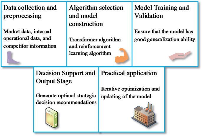
Based on the content of Fig. 1, data collection and preprocessing form the foundation of the entire model design. To ensure the comprehensiveness and representativeness of the data, data related to strategic management are collected through various channels, including market data, internal corporate operation data, and competitor information. In terms of algorithm selection and model construction, this work employs Transformer algorithms and RL algorithms. Model training and validation are critical steps in the model design, ensuring the model has good generalization capability. In the decision support and output stage, the trained model can make real-time predictions and analyses on new input data, generating optimal strategic decision recommendations. Finally, in the practical application process, new data are continuously collected, and the model is iteratively optimized and updated to ensure its ongoing adaptability to changing environments.
Table 2 lists the input and output variables.
Construction of the algorithm model
This work employs modern Transformer models and RL algorithms to address complex strategic decision-making problems. The Transformer model, a deep learning architecture that has achieved remarkable success in natural language processing in recent years, is primarily innovative due to its self-attention mechanism. This mechanism efficiently captures long-term dependencies in sequence data24. The Transformer model consists of two parts: the encoder and the decoder. The encoder processes input data through multiple self-attention layers and feedforward neural network layers, while the decoder converts the encoder’s output into the final prediction results25. The self-attention mechanism is calculated using Eq. (1):
$$\text{Attention}(Q,K,V)=\text{Softmax}\left(\frac{Q{K}^{T}}{\sqrt{{d}_{k}}}\right)V$$
(1)
\(Q\), \(K\), and \(V\) represent the query, key, and value matrices, respectively, and \({d}_{k}\) is the dimension of the key.
The Gaussian Error Linear Unit (GELU) activation function, defined as Eq. (2), is used:
$$f(x)=x\cdot\Phi (x)$$
(2)
\(\Phi\) is the cumulative distribution function of the standard normal distribution.
Cross-entropy loss is used to measure the discrepancy between the predictions and the actual labels, defined as Eq. (3):
$$L=-\sum_{i=1}^{N} {y}_{i}log\left({\widehat{y}}_{i}\right)$$
(3)
\({y}_{i}\) is the actual label and \({\widehat{y}}_{i}\) is the predicted probability.
RL is a learning method based on reward and punishment mechanisms, particularly suitable for scenarios requiring dynamic decision-making26,27. The primary algorithm used is the DQN28. The core of the Q-learning algorithm is the Q-function, which evaluates the long-term return of taking a specific action in a given state29,30. The Q-value update is defined by Eq. (4):
$$Q\left( {s_{t} ,a_{t} } \right) \leftarrow Q\left( {s_{t} ,a_{t} } \right) + \alpha \left[ {r_{t + 1} + \gamma \mathop {\max }\limits_{{a^{\prime } }} Q\left( {s_{t + 1} ,a^{\prime } } \right) – Q\left( {s_{t} ,a_{t} } \right)} \right]$$
(4)
\({s}_{t}\) is the current state, \({a}_{t}\) is the action taken, \({r}_{t+1}\) is the reward received, \(\gamma\) is the discount factor, and \(\alpha\) is the learning rate.
To ensure training stability and sample diversity, the experience replay mechanism configures a replay buffer capacity of 100,000 records. During each iteration, 64 samples (mini-batch) are randomly sampled for network training, with a sampling frequency of once per training step. By disrupting temporal correlations, experience replay mitigates high interdependencies among samples, thus enhancing model generalization ability and convergence speed.
A deep neural network is used to approximate the Q-function. The network training employs an experience replay mechanism to enhance training stability31,32. To combine the strengths of Transformer models and RL algorithms, this work proposes a hybrid optimization strategy. The Transformer model is used for feature extraction from input data to capture complex dependencies in sequence data, while the RL algorithm dynamically optimizes decisions based on these extracted features33,34. During the optimization process, the features generated by the Transformer model are used for RL state representation, and the RL algorithm adjusts the decision strategy based on these states35,36.
The model workflow is shown in Fig. 2:

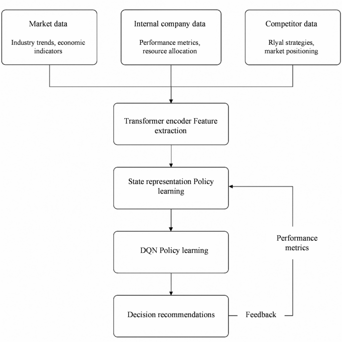
The workflow of the model.
In Fig. 2, the framework forms a complete dynamic learning loop, encompassing data input, feature encoding, policy learning, and output recommendation with feedback updates. The Transformer module extracts long-term dependencies in market trend features. The DQN module performs action selection and policy updates based on the state space, enabling dynamic generation of strategic optimization recommendations.
This work incorporates three categories of strategy-relevant data: market data (e.g., industry growth rate, customer demand shifts, macroeconomic indicators); internal corporate data (e.g., financial statements, employee turnover rate, product gross margins); competitor data (e.g., market share fluctuations, patent counts, public financing events). They are heterogeneous, multi-dimensional raw datasets.
A unified feature engineering process is first adopted to transform the data into structured numerical features for algorithmic modeling. Time-series variables (e.g., monthly sales, quarterly profits) preserve temporal ordering as Transformer model inputs. Categorical variables (e.g., competitive strategy types) are processed via one-hot encoding or embedding vectors. Continuous variables (e.g., market share) are normalized before direct model input. The features are ultimately encoded into high-dimensional dense vectors as input sequences for the Transformer. Through self-attention mechanisms, the Transformer extracts critical dependency relationships and outputs a composite state vector serving as the “environment state” for RL’s DQN.
The DQN selects optimal “actions” (strategies) based on the current state. These actions are designed as concrete strategic recommendations, including increasing budget allocation for specific business lines, adjusting human resource deployment, entering emerging markets next quarter, and engaging in price competition with rivals. The final output actions are mapped into natural language strategic recommendation reports for executive decision-making. This “strategy suggestion” process incorporates actual corporate feedback (e.g., profit changes, customer satisfaction variations) as reward signals for subsequent reinforcement learning iterations.
Algorithm optimization
In the process of algorithm optimization, this work employs several advanced optimization strategies to enhance the performance of the transformer model and RL algorithm. First, adaptive learning rate adjustment is a technique for dynamically adjusting the learning rate. Traditional fixed learning rates can lead to slow or unstable convergence during model training37,38. To address this issue, this work utilizes an adaptive learning rate algorithm. The Adam optimizer combines the momentum method and adaptive learning rate adjustment, adjusting each parameter’s learning rate by computing the first-order and second-order moment estimates of the gradient. The update rules of the Adam optimizer are given by Eqs. (5–9):
$${m}_{t}={\beta }_{1}{m}_{t-1}+\left(1-{\beta }_{1}\right){g}_{t}$$
(5)
$${v}_{t}={\beta }_{2}{v}_{t-1}+\left(1-{\beta }_{2}\right){g}_{t}^{2}$$
(6)
$${\widehat{m}}_{t}=\frac{{m}_{t}}{1-{\beta }_{1}^{2}}$$
(7)
$${\widehat{v}}_{t}=\frac{{v}_{t}}{1-{\beta }_{2}^{t}}$$
(8)
$${\theta }_{t+1}={\theta }_{t}-\frac{\eta {\widehat{m}}_{t}}{\sqrt{{\widehat{t}}_{t}+\epsilon }}$$
(9)
\({m}_{t}\) and \({v}_{t}\) are the momentum and variance estimates of the gradient, respectively. \({\beta }_{1}\) and \({\beta }_{2}\) are the momentum decay factors, \(\eta\) is the learning rate, and \(\epsilon\) is a smoothing term to prevent division by zero.
Compared to traditional optimization methods with fixed learning rates (e.g., Stochastic Gradient Descent), the Adam optimizer exhibits superior ability in dynamically adjusting parameter update magnitudes, particularly suitable for high-dimensional complex networks. In practical training, the Adam optimizer allocates adaptive learning rates to individual parameters based on gradient variation scales. Thus, it can accelerate early-stage convergence speed, reduce oscillation phenomena, and enhance final training stability. This approach enables the model to reach optimal ranges more efficiently while effectively decreasing iteration cycles and loss fluctuations.
Next, the hybrid optimization strategy leverages the strengths of both the transformer model and the RL algorithm. To optimize the hyperparameters in the transformer model, this work employs Bayesian Optimization. Bayesian Optimization guides the selection of hyperparameters by establishing a probabilistic model (Gaussian process) of the hyperparameter space39,40. The core of the optimization process lies in using the established probabilistic model to predict the performance of hyperparameter configurations and then selecting the optimal configuration through an exploration–exploitation strategy41. The objective function of Bayesian Optimization is given by Eq. (10):
$$\text{Objective Function }=\underset{\theta }{max} {\mathbb{E}}_{\text{model }}[f(\theta )]$$
(10)
\(\theta\) represents the hyperparameters, and \({\mathbb{E}}_{\text{model }}[f(\theta )]\) is the expected performance under the hyperparameter configuration.
In contrast to traditional grid search and random search methods, Bayesian optimization introduces prior knowledge and probabilistic prediction models to intelligently evaluate potentially optimal hyperparameter configurations within the search space. During model parameter tuning, Bayesian optimization typically locates near-optimal solutions with fewer trials, thus reducing tuning duration while improving precision. This methodology proves particularly advantageous for high-dimensional parameter spaces and computationally expensive training scenarios, such as selecting the number of attention heads and hidden layer dimensions in Transformer architectures.
Bayesian optimization employs Gaussian processes to model the hyperparameter space. The prior distribution adopts the common Radial Basis Function because it can capture the smooth changes in the input space. This work selects expected improvement as the acquisition function to guide optimization, effectively balancing exploration and exploitation to ensure focused searching in potentially optimal regions. The optimization procedure executes 100 iterations to progressively identify optimal hyperparameter combinations. During each iteration, the model updates based on current prior knowledge and experimental results, ultimately selecting the optimal configuration.
In the optimization of the RL algorithm, a multi-objective optimization (MOO) strategy is adopted, utilizing the Non-dominated Sorting Genetic Algorithm II (NSGA-II) to optimize the multi-objective function of the policy42,43. In this work, NSGA-II incorporates three optimization objectives: profit growth rate enhancement, customer satisfaction maximization, and resource consumption cost minimization. Each strategic action (e.g., market share adjustment or workforce allocation) corresponds to a three-dimensional objective function value.
NSGA-II generates multiple solution sets through population initialization and non-dominated sorting, while maintaining diversity via crowding distance computation. During iterations, the Pareto frontier progressively approaches optimal boundaries, with the solution closest to the ideal point ultimately selected for model policy updates. This methodology achieves balanced resource allocation and strategic recommendations under multiple competing objectives.
NSGA-II ranks different objectives of the policy and selects the optimal policy using the crowding distance44,45. The optimization process is described by Eqs. (11) and (12):
$$\text{NSGA}-\text{II Optimization}=\text{Pareto Front}$$
(11)
$$\text{Objective}={\text{min}}_{i}({\text{Cost}}_{i})$$
(12)
\(\text{Pareto Front}\) represents the Pareto frontier under multiple objectives, and \({\text{Cost}}_{i}\) is the cost of the i-th objective function.
NSGA-II, as a classical MOO method, can generate non-dominated solution sets when handling conflicting objectives in strategy selection (e.g., profit maximization versus cost minimization), from which Pareto-optimal strategies can be selected. During policy training, by incorporating crowding distance and rank sorting mechanisms, the algorithm effectively avoids local optima, thereby achieving a balance between solution diversity and global optimality. Particularly in complex market environments, NSGA-II enables decision-makers to evaluate trade-offs among multiple objectives, providing more robust policy references for RL.
Lastly, for the hybrid optimization of the transformer model and the RL algorithm, ensemble learning methods are introduced to integrate the results of different optimization algorithms46,47. By performing a weighted average of the prediction results from the transformer model and RL algorithm at different stages, the overall performance of the model is further enhanced48. The weighted equation for ensemble learning is given by Eq. (13):
$$\widehat{y}={\alpha }_{1}{\widehat{y}}_{1}+{\alpha }_{2}{\widehat{y}}_{2}$$
(13)
\({\widehat{y}}_{1}\) and \({\widehat{y}}_{2}\) are the prediction results of the transformer model and the RL algorithm, respectively, and \({\alpha }_{1}\) and \({\alpha }_{2}\) are the corresponding weights.
link